
Services
Introduction to Statistical Power
Below is an introduction to the concept of statistical power, a term you likely have heard in the context of designing a clinical study and planning the number of participants required to address the primary objective of the study.


Figure 1
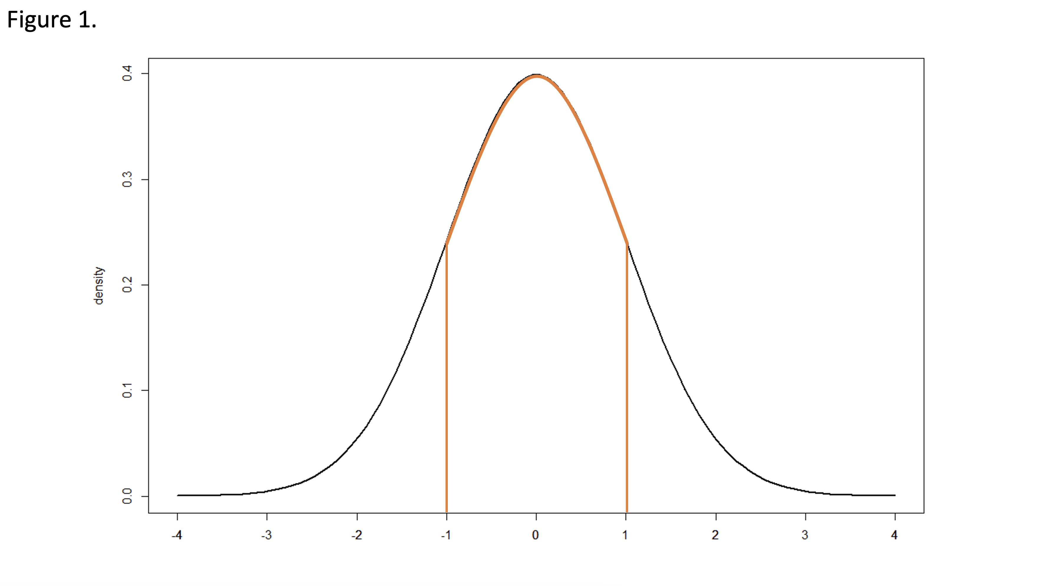
Figure 1 presents the standard normal distribution with a mean of zero and a standard deviation of 1. The probability density for a continuous variable is the probability per unit length. The probability density at a single point will equal 0. The cumulative probability density over a range of values will be greater than 0 and computed as the integral of the probability density function over the designated interval, equaling the area under the curve.
For example, in Figure 1, if we look at the probability that z equals -1, the probability will equal 0. We can instead look at the probability of z falling between -1 and 1. This value is non-zero and is equal to the area under the normal curve falling below and within the orange boundaries. The area is approximately 0.6826.
Figure 2
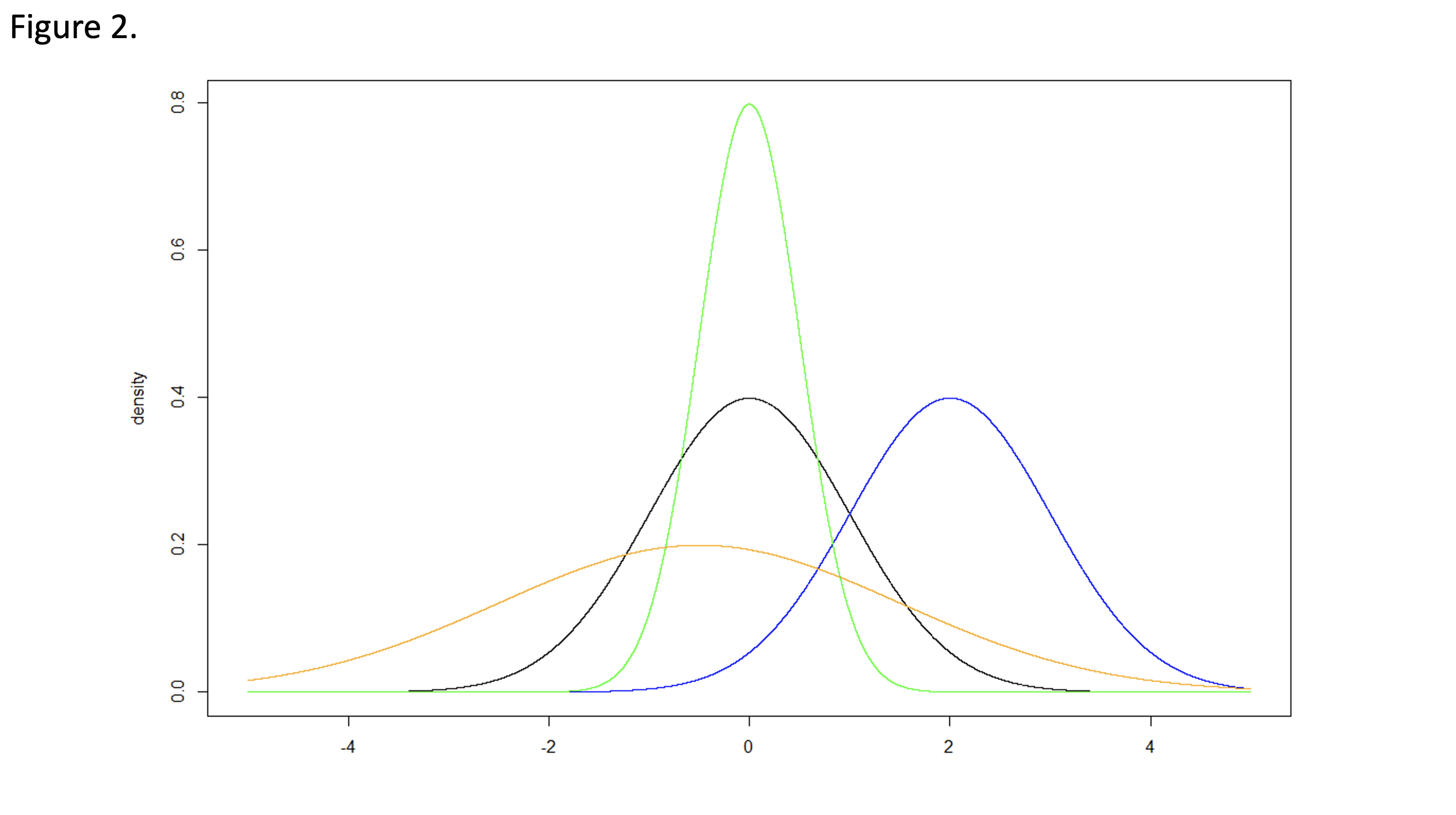
The standard normal distribution is convenient because the mean equals 0, the standard deviation equals 1, and many calculations therefore become straightforward. The same concepts can be extended to location shifts and scaling of the normal distribution. Figure 2 illustrates four normal distributions with varying location (i.e., mean values) and scale (i.e., standard deviations)
Figure 3
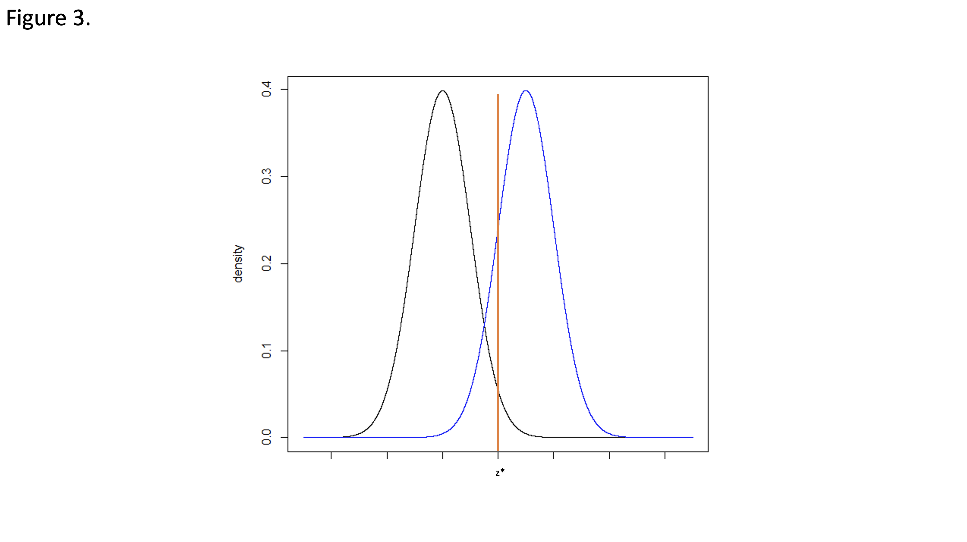
For simplicity, Figure 3 illustrates two identical normal distributions with a location shift so that the means are different (µ0 and µ1). The standard deviations are equivalent.
Consider a one-sided null hypothesis: H0: µ0 ≥ µ1 compared to the alternative hypothesis: HA: µ0 < µ1. The Type 1 error rate, α, is the probability of falsely rejecting the null hypothesis under the condition that the null hypothesis is true. Using the normal distributions in Figure 3, we can identify the critical value z* for a one-sided hypothesis test, corresponding to the upper 100*α% of the null distribution where the null hypothesis is rejected. When performing a statistical hypothesis test, we would interpret any value falling above z* would be unlikely to come from the null distribution. If the null hypothesis is true, this would be a “false positive.”
The Power of the study is the cumulative density of the alternative hypothesis probability function, centered µ1, that falls above the critical value z*. Values above z* allow us to reject the null hypothesis. If the null hypothesis is false and the alternative hypothesis is true, we want to have a high probability of rejecting the null hypothesis. Therefore, when designing a study, we would typically plan for a high power, often 80% or 90%.
The Type 2 error rate is equal to 1-power. It is the probability of falsely failing to reject the null hypothesis under the condition that the alternative hypothesis is true. In Figure 3, the type 2 error rate, or β, is the cumulative probability density of the alternative distribution that falls below z*.
-
Let's Talk.
Contact Veristat Today!We know there are always unknown challenges when bringing a novel therapeutics to market, so we’ve assembled an extraordinary team of scientific minded experts who have mastered the complexities of therapeutic development enabling sponsors to succeed in extending and saving lives.
Introduction to Sample Size, Standard Deviation, and Power
When planning a study, researchers must determine the number of participants required for analysis of the primary endpoint to address the primary objective of the study, but what is an appropriate sample size?
Figure 4
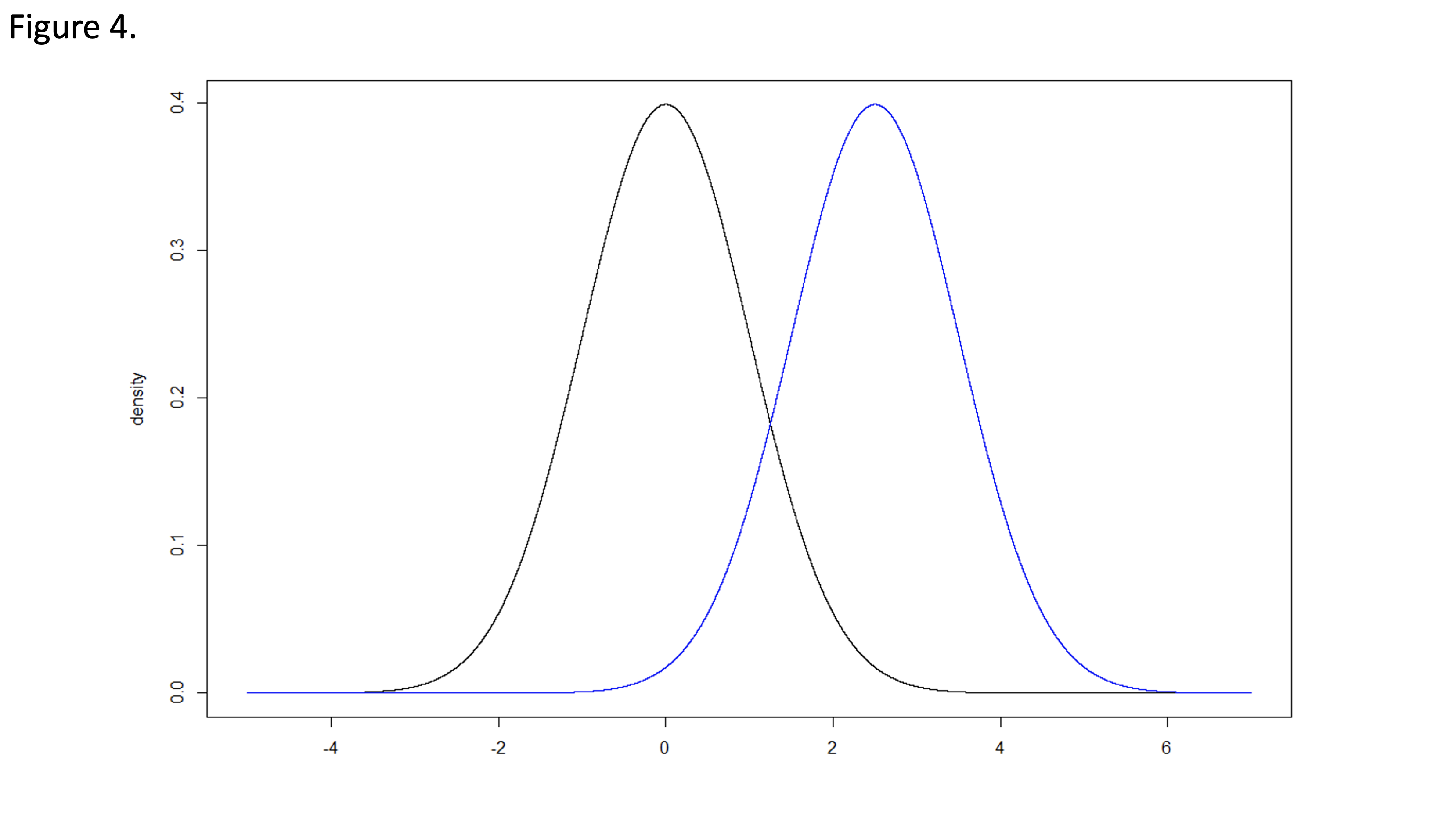
Consider two normal distributions with means µ0 and µ1 and standard deviations equal to 1. (Figure 4) We can test a one-sided null hypothesis: H0: µ0 ≥ µ1 compared to the alternative hypothesis: HA: µ0 < µ1. The type I error rate (α) is the probability of rejecting the null hypothesis under the condition that the null hypothesis is true. The power (1-β) is the probability of correctly rejecting a false null hypothesis. This document focuses on the normal distribution, though the same concepts can be directly transferred to any other distribution or applied statistic.
An appropriate sample size is selected to ensure a high probability of failing to reject the null hypothesis if it is true, and to reject the null hypothesis if it is false. The sample size can be computed as a function of the type I error rate, power, and standard deviation of the sample. The type I error rate and power can be selected a priori and are fixed values for the design of the study. The hypothesized means and differences in means are assumptions made for the design of the study. The sample size will be selected to provide sufficient precision of the estimated means in order to achieve the targeted power and type I error rate under the assumptions made during study planning.
Figure 5a
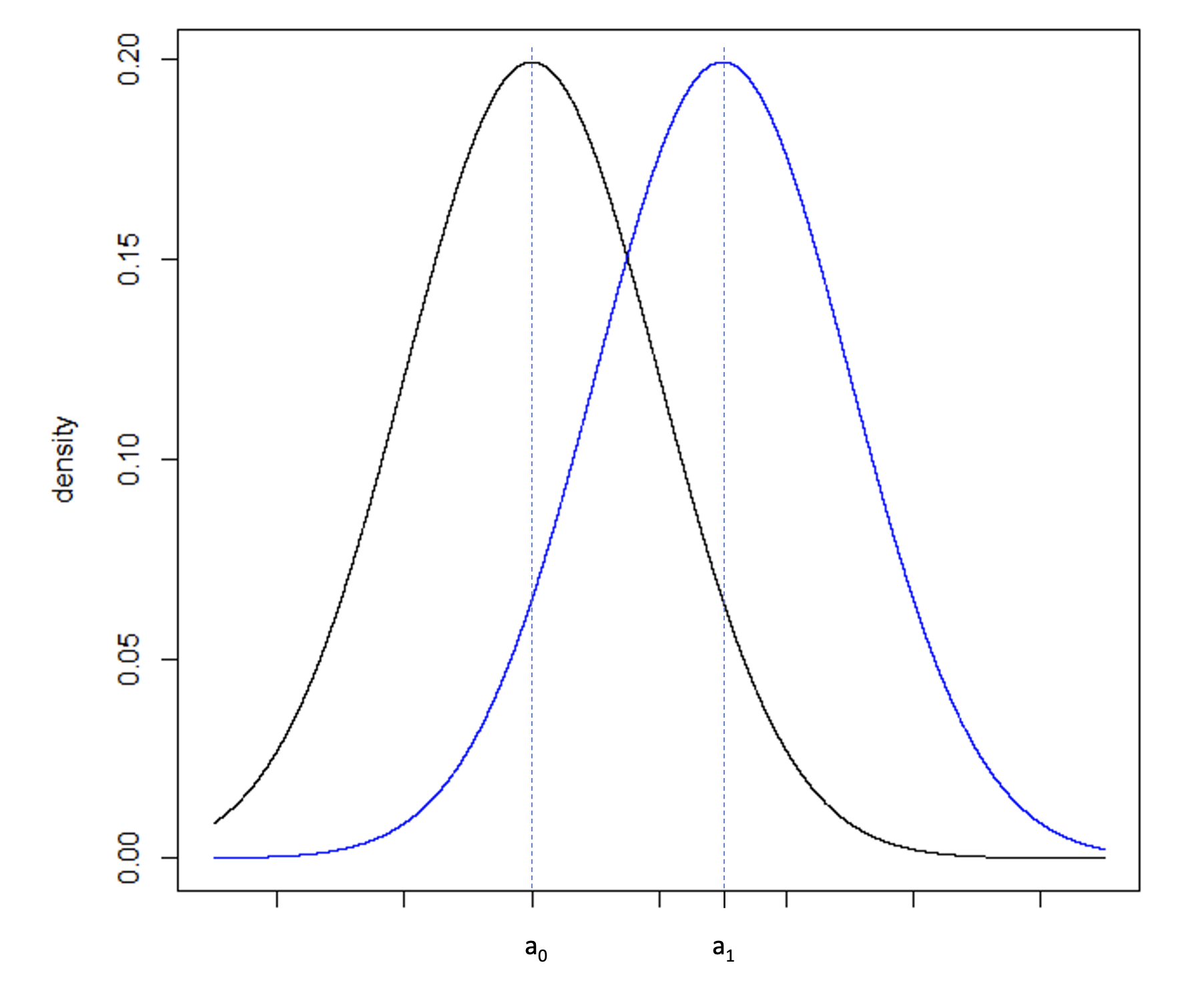
Figure 5b
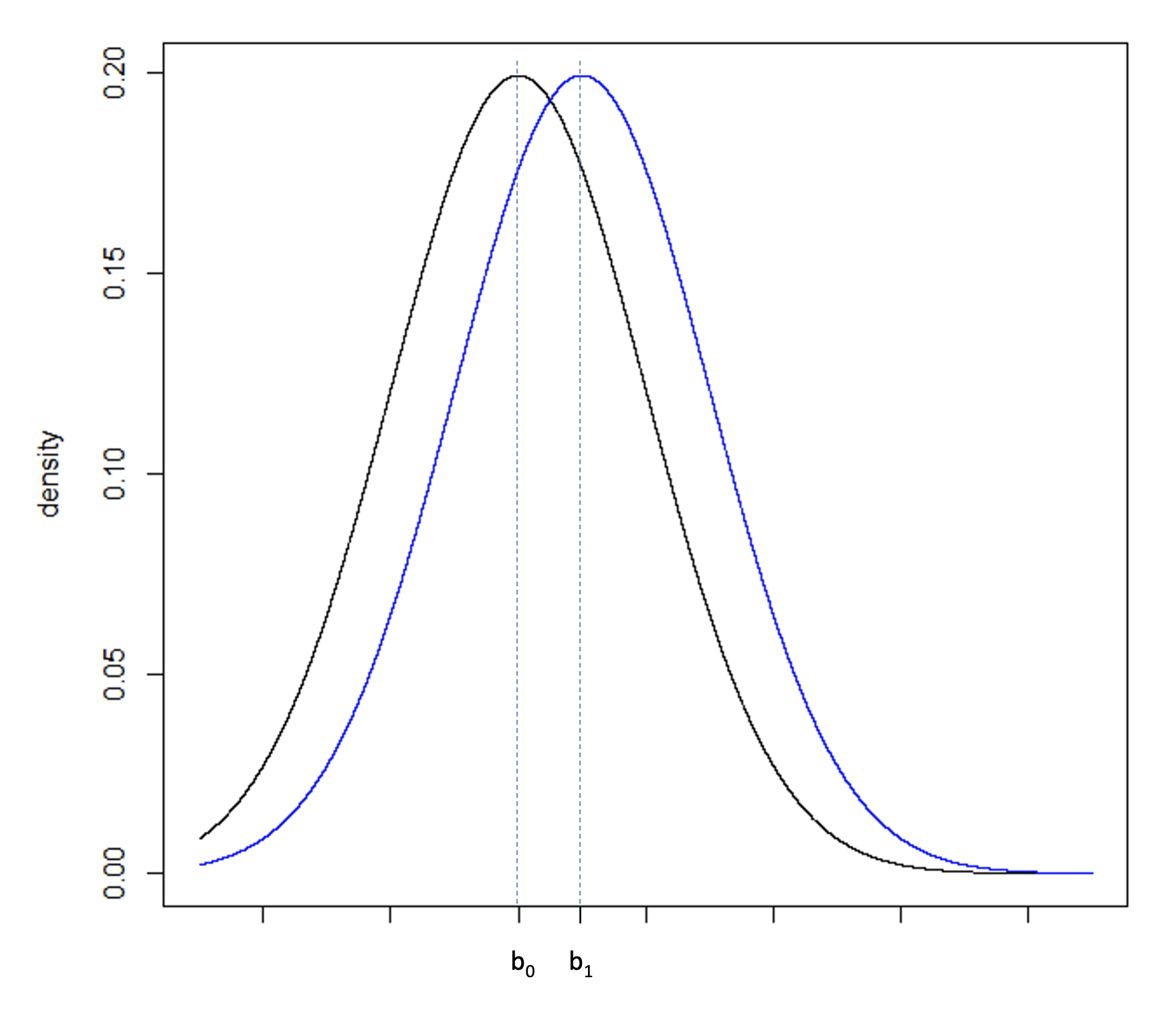
Figure 5c
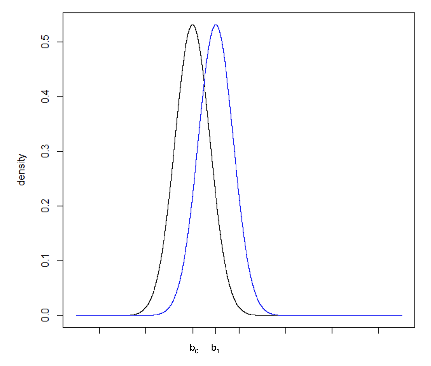
Consider Figure 5a, illustrating two normal distributions with a0 and a1 having a large difference compared to Figure 5b where b0 and b1 fall closer together. The underlying standard deviation expected from each distribution is the same. In Figure 5a, the standard deviation is small in comparison to the difference between a0 and a1. In Figure 5b, the standard deviation is large in comparison to the smaller difference between b0 and b1. To increase the power of a hypothesis test of the null and alternative hypothesis: H0: b0 ≥ b1 vs. HA: b0 < b1, the precision of the sample estimate must be increased, which can be achieved by increasing the sample size, and therefore reducing the standard error of the sample, Figure 5c.
Standard error = Standard deviation/ square root of the sample size.
Given these relationships, an adjustment of the sample size can be used to control the relative precision of the sample estimates and therefore can influence the power of the study.
When planning a study, the type I error rate is typically determined prior to sample size calculations and captures the risk of moving forward under a “false positive” condition. While exceptions exist, for early phase clinical studies (i.e., Phase 1), a one-sided type I error rate may be more lenient, e.g., 5% or 10%, whereas a later phase clinical study (i.e., Phase 3), the one-sided type I error rate will typically be smaller, e.g., 2.5%. The power of a later phase study is typically targeted to be between 80% or 90%. During the study design and sample size calculation, sample sizes can be computed for a series of values for µ0 or µ1 and assumed standard deviations.
The balance of sample size versus standard deviation versus mean versus power can be an extensive conversation when designing a study and should be based on prior research either in clinic or that is available in literature, as well as considering what are clinically meaningful differences to select an observable difference with a sufficient precision to allow reasonable conclusions from a newly designed study.
Statistical Power and Minimum Detectable Differences
Concepts of statistical power and its relationship to a minimum detectable difference are relevant when planning a new study. They can inform how and when researchers might observe a statistically significant difference between two values and can be used to better inform sample size selection during protocol development.
The two values could be the difference in means or proportions between two treatment groups or could be a comparison of either a mean or a proportion to a predefined constant. This document focuses on the normal distribution, though the concepts discussed can be directly transferred to any other distribution or applied statistic.
Consider a one-sided null hypothesis: H0: µ0 ≥ µ1 compared to the alternative hypothesis: HA: µ0 < µ1.
Figure 6
The Type 1 error rate (α), is the probability of falsely rejecting the null hypothesis under the condition that the null hypothesis is true. Using the normal distributions in Figure 6, we can identify the critical value z* for a one-sided hypothesis test, corresponding to the upper 100*α% of the null distribution where the null hypothesis is rejected. When performing a statistical hypothesis test, we would interpret any value falling above z* would be unlikely to come from the null distribution. If the null hypothesis is true, this would be a “false positive”.
The Power of the study is the probability of correctly rejecting a false null hypothesis, also known as the cumulative density of the alternative hypothesis probability function, centered µ1, that falls above the critical value z*. Values above z* allow us to reject the null hypothesis. If the null hypothesis is false and the alternative hypothesis is true, we want to have a high probability of rejecting the null hypothesis. Therefore, when designing a study, we would typically plan for a high power, often 80% or 90%.
If we consider the critical value, z*, we can see that any values above z* are statistically significant. When we are designing the study, we may want to know the minimum detectable difference, the minimum magnitude of difference that needs to be observed in order to have a statistically significant result. It is important to ensure this value corresponds to a relevant difference that is clinically meaningful. If, for example, the difference observed in a new drug clinical study is very small but statistically significant due to large sample size and low standard deviation, this may not be a meaningful improvement over the already available therapy and therefore is not a meaningful difference to observe.
To determine the minimum detectable difference, we can use the critical value from the standard normal distribution (Z-score) and translate this value to the scale of the observed sample values to understand how big of a difference is required to observe a statistically significant result under the assumed null value, type I error rate, and standard deviation.
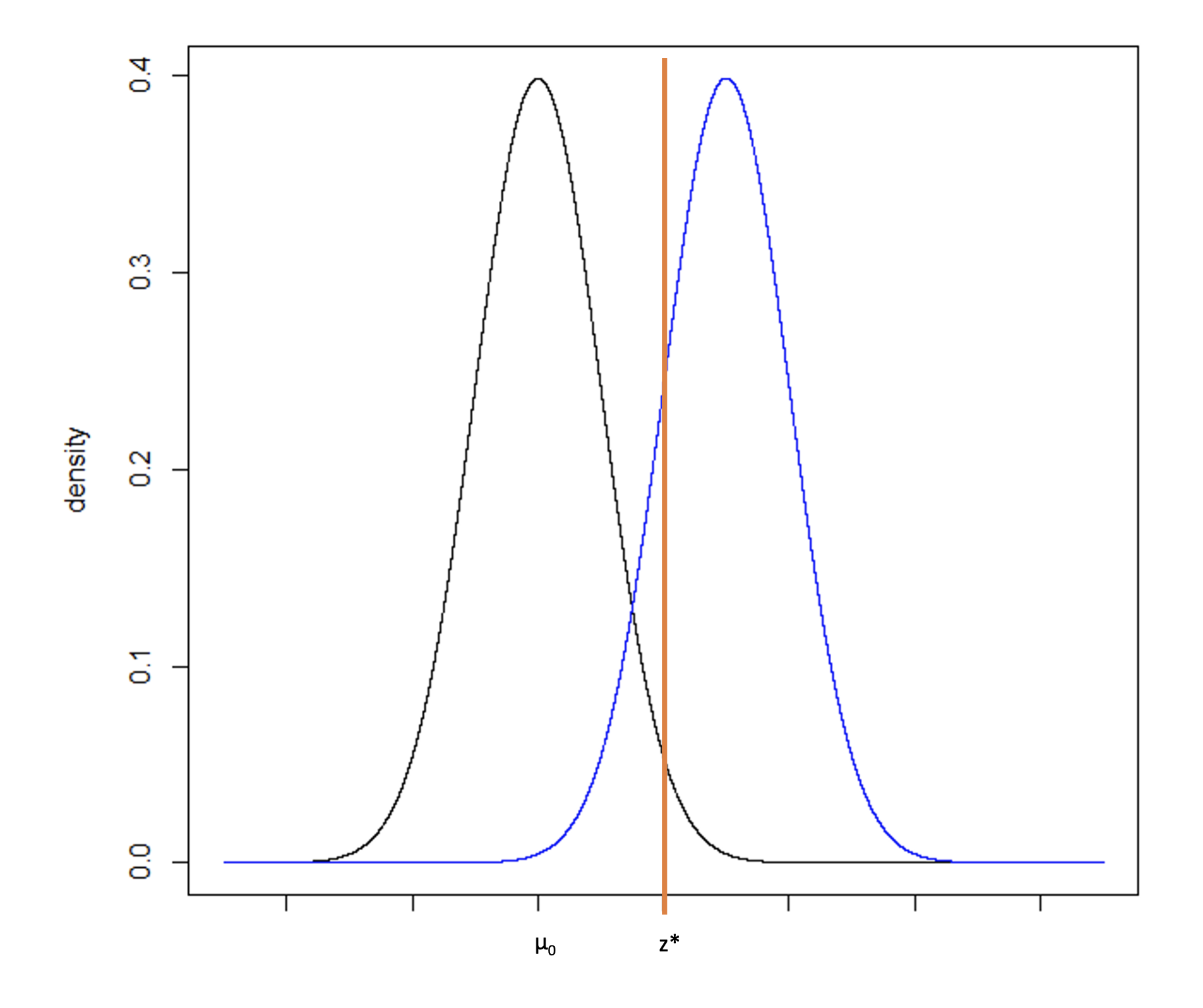
Figure 7
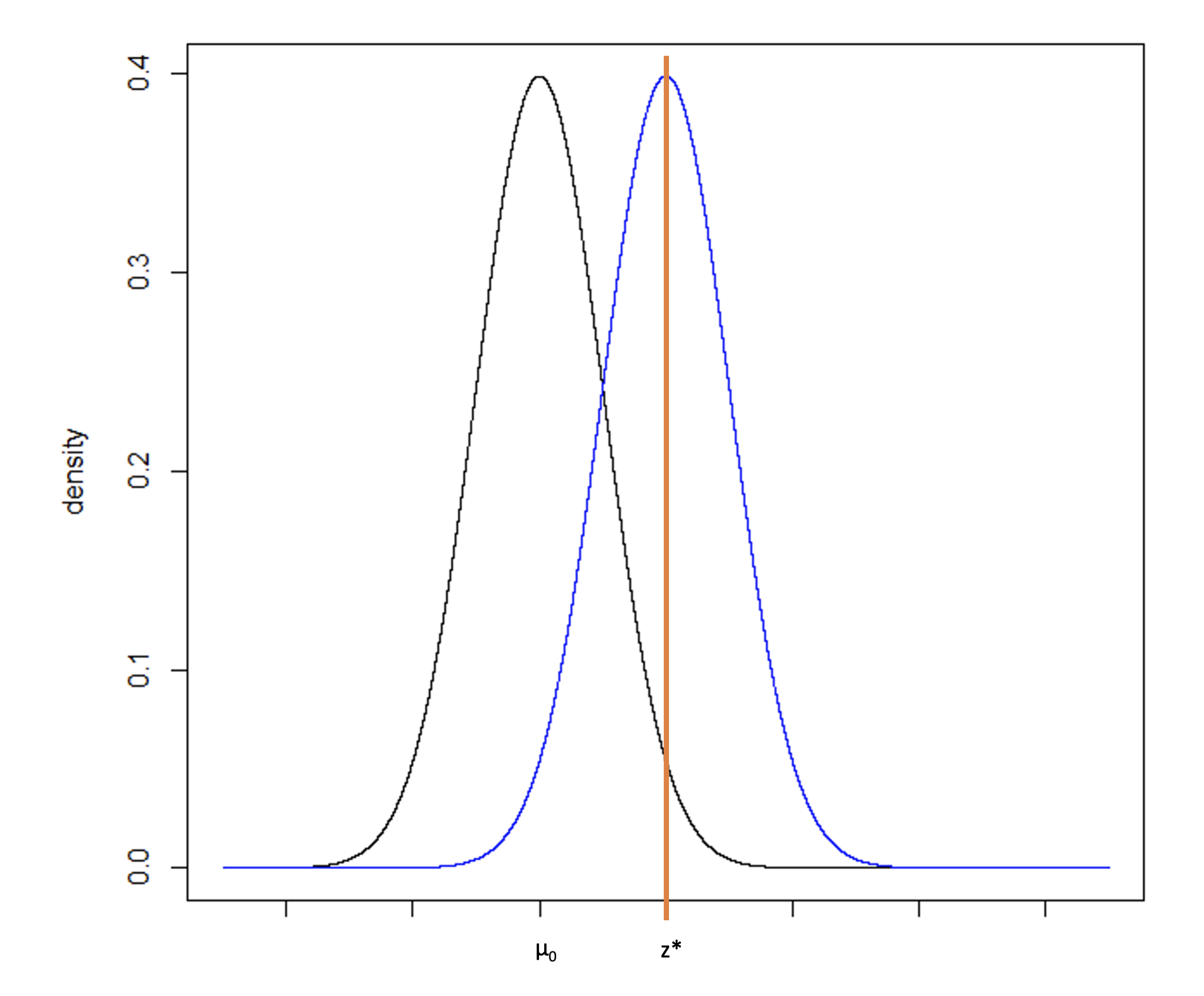
While the translation from the normal distribution to a difference in means (for example) is a straightforward calculation, sometimes test statistics are difficult to back-transform and the calculation is not obvious. As an alternative approach, we can consider Figure 7 with two normal distributions, one centered on µ0 and one centered on z*. Recall that power is equal to the probability of rejecting the null hypothesis if the alternative hypothesis is true. It is computed as the cumulative probability density falling above the critical value, z*.
The sample size was determined given a set type I error rate, power, hypothesized difference (between µ0 and µ1), and standard deviation. To determine the critical value, we will keep the sample size, type I error rate, and standard deviation constant but will reduce the power to 50%. From sample size software we can compute the difference that would be required to provide 50% power, which is equivalent to an alternative hypothesis centered at the critical value z*. This is the minimum detectable difference that can be observed with a statistically significant p-value under the assumed sample size, type I error rate, and standard deviation.
Learn More with These Resources

Fact Sheet
Data-Driven Strategies to Advance Development and Approval of ...

Infographic
Four Pillars of Success in Neurology Trials

Case Study
Advancing Oncology Innovation